 | Lecture 10. Predation and parasitism |
Parasitoids. This wasp is laying its egg inside an aphid where its young will develop. Parasitoid immatures develop on or inside a host, killing it as they mature. They emerge as adults and continue the cycle |
Predators. Lady beetles are well-known examples of predatory insects. A predator consumes many prey during its lifetime. The predators listed in this guide feed on insects and mites. |
Pathogens. This nematode is just one example of a pathogen which may kill its host. Other pathogens include bacteria, viruses, fungi and protozoa. This section also includes antagonists which control plant diseases. |
Weed Feeders. Weeds can be attacked by arthropods, vertebrates, and pathogens (fungi, viruses, bacteria, and nematodes). This weevil feeds only on one particular type of weed called purple loosestrife. |
F1.Lotka-Volterra model |
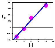
F2. Keep constant density of prey (e.g., H = 0, 5, 10, 20, 100 prey/cage), and estimate the intrinsic rate of predator population increase (rP) at these densities of prey. Plot the intrinsic rate of predator population increase versus prey density: The linear regression of this line is: |
|
F3 - the Euler''s method |
F4 |
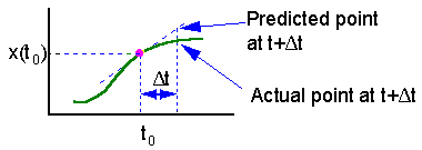
On this graph we estimate the slope f(x) of the function at point t = to and extrapolate this slope through the entire time interval |
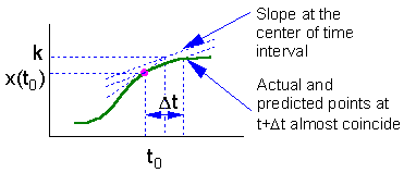
F5 -estimating the derivative at the middle point,k is the function value in the center of time interval l (F6) |
F6. Finally, we can estimate function value at the end of the time interval: |
|
This is called Runge-Kutta method of second order. The most popular is the Runge-Kutta method of the fourth order. However, for our purposes it is enough to use the second order method.This method is applied to Lotka-Volterra equations in the following Excel spreadsheet -http://home.comcast.net/~sharov/PopEcol/xls/lotka.xls, First, we estimate prey and predator densities (H'' and P'', respectively) at the center of time interval |
The second step is to estimate prey and predator densities (H" and P" at the end of time step l (F6) |
|
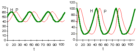
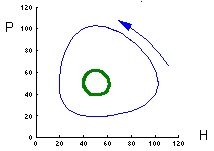
These two graphs were plotted using the same model parameters. The only difference is in initial density of prey. This model has no asymptotic stability, it does not converge to an attractor (does not "forget" initial conditions). |
This figure shows relative changes in prey predator density for both initial conditions. Trajectories are closed lines. |
F7 - Assume that a predator captured Ha prey during time T. Handling time should be proportional to the number of prey captured: |
where Th is time spent on handling of 1 prey. |
F8, hence |
Now we can balance the time budget |
F9 |
F10, where Th is time spent on handling of 1 prey. |
F11, Hence: |
Now we can balance the time budget: |
The last step is to find the number of attacked prey Ha |
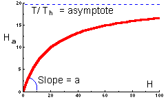
The graph of functional response that corresponds to this equation is shown below |
This function indicates the number of prey killed by 1 predator at various prey densities. This is a typical shape of functional response of many predator species. At low prey densities, predators spend most of their time on search, whereas at high prey densities, predators spend most of their time on prey handling. |
|
F13 |
F14 |
F15 |
10.3. Functional and Numerical Response
10.4. Predator-Prey Model with Functional Response
10.5. Host-Parasitoid Models
10.6. Host-Pathogen Model (Anderson & May)
Predation and parasitism are examples of antagonistic ecological interactions in which one species takes advantage of another species. Predators use their prey as a source of food only, whereas parasites use their hosts both as a food and as a habitat. Predation and parasitism are stage-specific interactions rather than species-specific. Many species are predators or parasites only on specific stages in their life cycle.
Importance of the study of predation and parasitism:
� In many species predation and parasitism are dominating among ecological processes. Dynamics of these populations cannot be predicted and understood without considering natural enemies.
� Pest species of insects and weeds can be suppressed by introduction of natural enemies or by inundative release of natural enemies (biological control).
� Natural enemies may cause side effects in pesticide applications. The numbers of arthropod natural enemies may be reduced due to pesticide treatment which may result in increasing of pest populations.
10.2 Lotka-Volterra Model
Lotka-Volterra model is the simplest model of predator-prey interactions. The model was developed independently by Lotka (1925) and Volterra (1926) F1.
It has two variables (P, H) and several parameters:
H = density of prey
P = density of predators
r = intrinsic rate of prey population increase
a = predation rate coefficient
b = reproduction rate of predators per 1 prey eaten
m = predator mortality rate
Measuring parameters of the Lotka-Volterra model
The following set of experiments should be done:
1. Keep prey population without predators and estimate their intrinsic rate of increase (r).
2. Put one predator in cages with different densities of prey and estimate prey mortality rate and corresponding k-value in each cage. As we know, k-value equals to the instantaneous mortality rate multiplied by time. Thus, the predation rate (a) equals to the k-value divided by the duration of experiment.
Example: lady-beetle killed 60 aphids out of 100 in 2 days. Then, the k-value = -ln(1-60/100) = 0.92, and a = 0.92/2 = 0.46.
Note: if a -values estimated at different prey densities are not close enough to each other, then the Lotka-Volterra model will not work! However, the model can be modified to incorporate the relation of a to prey density.
3. Estimation of parameters b and m F2.
1. Note: If points do not fit to a straight line (e.g., the intrinsic rate of predator population growth may level off), then the Lotka-Volterra model is not adequate and should be modified. Now , parameters b and m can be taken from this regression equation.
How to solve differential equations
There are two major approaches: analytical and numerical. Analytical methods are complicated and require good mathematical skills. Also, many differential equations have no analytical solution at all. Numerical methods are easy and more universal (however, there are problems with convergence).
The simplest and least accurate is the Euler''s method. Consider a stationary differential equation F3.
First we need initial conditions. We will assume that at time to the function value is x(to).
Now we can estimate x-values at later (or earlier) time using equation F4.
The main source of error in the Euler''s method is estimation of derivative at the start of time interval. The direction of actual solution may change drastically during this time interval and numerically predicted point could be far from the actual solution (see the figure).
Euler''s method can be improved, if the derivative (slope) is estimated at the center of time interval . However, the derivative at the center depends on the function value at the center which is unknown. Thus, first we need to estimate the function value at the middle point using simple Euler''s method, and then we can estimate the derivative at the middle point F5.
The model of Lotka and Volterra is not very realistic. It does not consider any competition among prey or predators. As a result, prey population may grow infinitely without any resource limits. Predators have no saturation: their consumption rate is unlimited. The rate of prey consumption is proportional to prey density. Thus, it is not surprising that model behavior is unnatural showing no asymptotic stability. However numerous modifications of this model exist which make it more realistic.
Modeling Functional Response
Holling (1959) suggested a model of functional response which remains most popular among ecologists. This model is often called "disc equation" because Holling used paper discs to simulate the area examined by predators. Mathematically, this model is equivalent to the model of enzime kinetics developed in 1913 by Lenor Michaelis and Maude Menten.
This model illustrates the principal of time budget in behavioral ecology. It assumes that a predator spends its time on 2 kinds of activities:
1. Searching for prey
2. Prey handling which includes: chasing, killing, eating and digesting.
Consumption rate of a predator is limited in this model because even if prey are so abundant that no time is needed for search, a predator still needs to spend time on prey handling.
Total time equals to the sum of time spent on searching and time spent on handling F7
Capturing prey is assumed to be a random process. A predator examines area a per time unit (only search time is considered here) and captures all prey that were found there. Parameter a is often called "area of discovery", however it can be called "search rate" as well.
After spending time Tsearch for searching, a predator examines the area = a Tsearch, and captures aHTsearch prey where H is prey density per unit area F8
10.3. Functional and Numerical Response
Holling (1959) studied predation of small mammals on pine sawflies, and he found that predation rates increased with increasing prey population density. This resulted from 2 effects: (1) each predator increased its consumption rate when exposed to a higher prey density, and (2) predator density increased with increasing prey density. Holling considered these effects as 2 kinds of responses of predator population to prey density: (1) the functional response and (2) the numerical response.
Modeling Functional Response
Holling (1959) suggested a model of functional response which remains most popular among ecologists. This model is often called "disc equation" because Holling used paper discs to simulate the area examined by predators. Mathematically, this model is equivalent to the model of enzime kinetics developed in 1913 by Lenor Michaelis and Maude Menten.
This model illustrates the principal of time budget in behavioral ecology. It assumes that a predator spends its time on 2 kinds of activities:
1. Searching for prey
2. Prey handling which includes: chasing, killing, eating and digesting.
Consumption rate of a predator is limited in this model because even if prey are so abundant that no time is needed for search, a predator still needs to spend time on prey handling.
Total time equals to the sum of time spent on searching and time spent on handling F9.
Assume that a predator captured Ha prey during time T. Handling time should be proportional to the number of prey captured F10
Capturing prey is assumed to be a random process. A predator examines area a per time unit (only search time is considered here) and captures all prey that were found there. Parameter a is often called "area of discovery", however it can be called "search rate" as well.
After spending time Tsearch for searching, a predator examines the area = a Tsearch, and captures aHTsearch prey where H is prey density per unit area F11
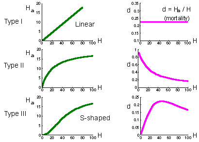
Holling (1959) considered 3 major types of functional response F12
Type I functional response is found in passive predators like spiders. The number of flies caught in the net is proportional to fly density. Prey mortality due to predation is constant (right graph on the previous page).
Type II functional response is most typical and corresponds to the equation above. Search rate is constant. Plateau represents predator saturation. Prey mortality declines with prey density. Predators of this type cause maximum mortality at low prey density. For example, small mammals destroy most of gypsy moth pupae in sparse populations of gypsy moth. However in high-density defoliating populations, small mammals kill a negligible proportion of pupae.
Type III functional response occurs in predators which increase their search activity with increasing prey density. For example, many predators respond to kairomones (chemicals emitted by prey) and increase their activity. Polyphagous vertebrate predators (e.g., birds) can switch to the most abundant prey species by learning to recognize it visually. Mortality first increases with prey increasing density, and then declines.
If predator density is constant (e.g., birds, small mammals) then they can regulate prey density only if they have a type III functional response because this is the only type of functional response for which prey mortality can increase with increasing prey density. However, regulating effect of predators is limited to the interval of prey density where mortality increases. If prey density exceeds the upper limit of this interval, then mortality due to predation starts declining, and predation will cause a positive feed-back. As a result, the number of prey will get out of control. They will grow in numbers until some other factors (diseases of food shortage) will stop their reproduction. This phenomenon is known as "escape from natural enemies" discovered first by Takahashi.
Estimation of Parameters of Functional Response
Experiments should be done as follows: predators are kept in large-size cages individually. Large-size cages are important because search abilities of predators should be limited. Different number of prey are released in these cages. Each prey density should be replicated to get sufficient accuracy. More experiments should be done with low prey density than with high prey density because the error of mortality estimates depends on the total number of prey. Experiments are usually set for a fixed time interval. At the end of experiments, survived prey are counted in each cage.
This is an example of experimental data:
No. of
prey per
cage
H No. of
replications Total
prey
killed Average no.
of prey killed
Ha 1/Ha 1/(HT)
5 20 50 2.5 0.400 0.1000
10 10 40 4.0 0.250 0.0500
20 7 55 7.9 0.127 0.0250
40 5 45 9 0.111 0.0125
80 3 38 12.6 0.079 0.0062
160 3 35 11.6 0.086 0.0031
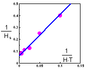
Cage area was 10 sq.m., and duration of experiment was T=2 days. Holling''s equation can be transformed to a linear form F13
The linear regression has the following coefficients F14:
y = 3.43 x + 0.0612
Th = 0.0612 T = 0.1224 days = 2.9 hours
a = 1/3.43 = 0.29 cages = 2.9 sq.m.
Another possible method of parameter estimation is non-linear regression. It may give better results at high prey density than the linear regression method.
Type III functional response can be simulated using the same Holling''s equation with search rate (a) dependent on prey density, e.g.F15
Numerical Response
Numerical response means that predators become more abundant as prey density increases. However, the term "numerical response" is rather confusing because it may result from 2 different mechanisms:
1. Increased rate of predator reproduction when prey are abundant (numerical response per se)
2. Attraction of predators to prey aggregations ("aggregational response")
Reproduction rate of predators naturally depends on their predation rate. The more prey consumed, the more energy the predator can allocate for reproduction. Mortality rate also reduces with increased prey consumption.
The most simple model of predator''s numerical response is based on the assumption that reproduction rate of predators is proportional to the number of prey consumed. This is like conversion of prey into new predators. For example, as 10 prey are consumed, a new predator is born.
Aggregation of predators to prey density is often called "aggregational response". This term is better than "numerical response" because it is not ambiguous. Aggregational response was shown to be very important for several predator-prey systems. Predators selected for biological control of insect pests should have a strong aggregational response. Otherwise they would not be able to suppress prey populations. Also, aggregational response increases the stabilility of the spatially-distributed predator-prey (or host-parasite) system.
http://home.comcast.net/~sharov/PopEcol/lec10/funcresp.html
Next: Predator-Prey Model
Main Text
Biological Control
Lotka-Volterra Model
Lotka-Volterra Two Species Model
