 | Trend Surface analysis and other statistical items in GIS |
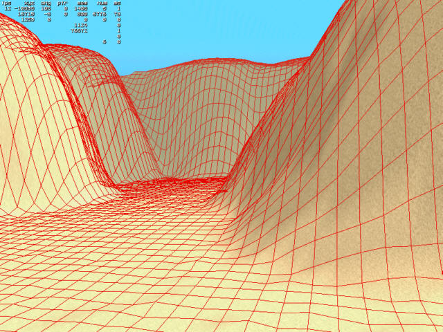
this 3D created with reducing a gravity trend |
Distance function |
Contour maps |
Performing trend analysis first - order polynomial |
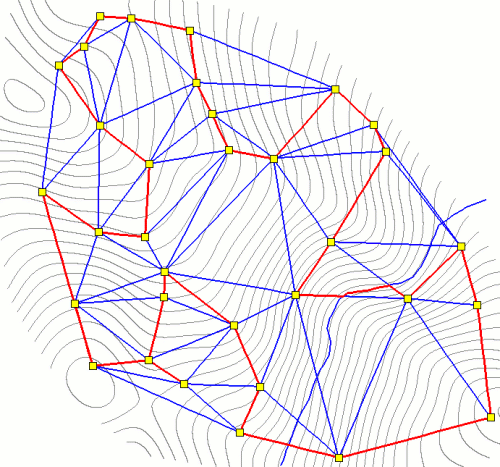
triessen polygons |
|
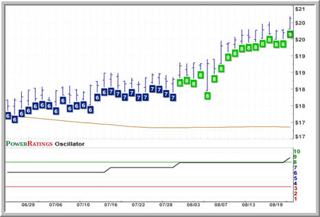
Moving averages |
200-day moving average. |
Trend sutface 3rd order polynomial |
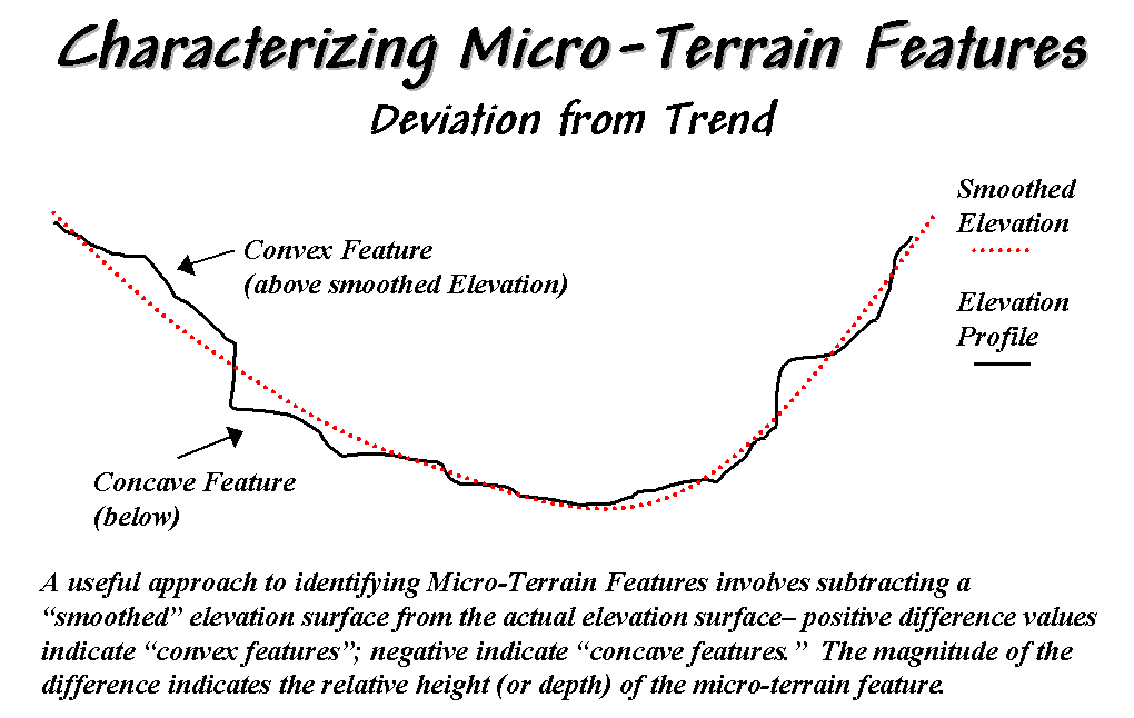
smoothing |
3D terrain Rendering |
Aspect-slope |
Aspect ratio GIS layer (compass direction of the facing slope). |
aspect |
#1 Countor map |
#2 a photograph from the summit viewpoint |
#3 the equivalent view generated from the terrain model. Here the vector map of the restocking proposals is draped over |
#4 Using the digitised terrain data, a DTM was created by a module of the GIS system |
#5 Having produced the DTM, various methods of visual analysis are possible. Slope, aspect or shade maps can be produced |
In addition to the 2-Dimensional maps described earlier, 3-Dimensional views can be derived from the DTM |
hillshading techniques |
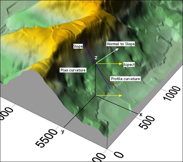
Curvature (profile, plan) and morphometric analysis - http://www.spatialanalysisonline.com/output/html/Curvatureandmorphometricanalysis.html |
slope.aspect |
Visibility analysis - http://webhelp.esri.com/arcgisdesktop/9.2/index.cfm?TopicName=Visibility_analysis |
Network analysis - http://www.esri.com/software/arcgis/extensions/networkanalyst/index.html |


Trend surfaces are widely used by geologists, particularly in petroleum exploration, as a means of separating a mapped variable into two components, the trend and the residuals from the trend. The trend corresponds to the concept of "regional features," while residuals represent "local features." Used in this manner, trend surface analysis is a global method for filtering spatial data.
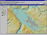
This plot shows Bouguer gravity data for northwest Kansas. While there are several interesting features, there is also a strong west-to-east trend.
There are a number of disadvantages to a global fit procedure. The most obvious of these is the extreme simplicity in form of a polynomial surface as compared to most natural surfaces. A first-degree polynomial trend surface is a dipping flat plane. A second-degree surface may have only one maximum or minimum. In general, the number of possible inflections in a polynomial surface is one less than the number of coefficients in the trend surface equation. As a consequence, a trend surface generally cannot pass through the data points, but rather has the characteristics of an average.
Polynomial trend surfaces also have an unfortunate tendency to accelerate without limit to higher or lower values in areas where there are no control points, such as along the edges of maps. All surface estimation procedures have difficulty extrapolating beyond the area of data control, but trend surfaces seem especially prone to the generation of seriously exaggerated estimates.
Computational difficulties may be encountered if a very high degree polynomial trend surface is fitted. This requires the solution of a large number of simultaneous equations whose elements may consist of extremely large numbers. The matrix solution may become unstable, or rounding errors may result in erroneous trend surface coefficients.
Nevertheless, trend surfaces are appropriate for estimating a grid matrix in certain circumstances. If the raw data are statistical in nature, with perhaps more than one value at an observation point, trend surfaces provide statistically optimal estimates of a linear model that describes their spatial distribution.
Distance function
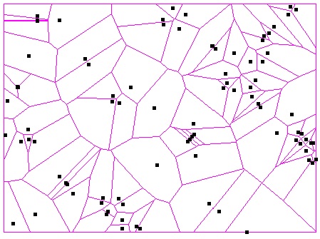
Global- and local-fit contouring procedures are appropriate for mapping surfaces that represent variables whose values are known at discrete observation points. In addition, Surface III will produce grids and maps that simply reflect the locations of the observation points themselves. They display distance functions which do not represent the values of a surface at all, but rather the distances from any location on the map to the locations of nearby control points. A distance function map is useful for assessing the reliability of a contour map made from the original data, as the contour map will obviously be of lower reliability in areas where control is most distant. Surface III can construct grids giving the distance to the nearest control point, the average distance to a specified number of control points, or the distance to the most distant of a specified number of points.
The following is an example of a typical distance function map. The contours show the distance from any point on the map to the nearest well (wells shown by plus symbols). The contour interval is 0.2 miles. Distance function maps also can be used to automatically define oil field boundaries, by drawing a single contour line a specified distance around all producing wells. Any phenomenon whose influence declines with distance may be analyzed by distance function maps.
Spatial relationships between sample points can be analyzed using the Distance Map option of Surface III. Among other applications, it can be used to investigate the effectiveness of different search methods with specific data sets. Distance Map will display the local density of control points in the form of contour maps of the distance from each grid node to some specified set of control points.
Other statistics related to the local subset of observations around each grid node also can be computed and displayed as maps. These include maps of the distances to the nearest, farthest, and average neighbors of a point, the standard deviations of distances to neighbors of a point, the number of neighboring observations within specified distances of a point, the number of octants or quadrants containing specified numbers of points, and measures of the relative contributions of the nearest, farthest, and average neighbors to the estimates of values at the grid nodes.
Performing trend analysis
Trend Surface Analysis
Trend Surface analysis
Surface
Trend Surface analysis