Integrated geological data management and analysis

Data Input/Management: The RockWorks data manager operates like a spreadsheet, reading and saving row and column data as ASCII tab-delimited files. Easy cut and paste from other applications. Special features include display of graphic symbols, colors, and line styles right in the data sheet, and hyperlinks to accessory files containing downhole data, graphic images, etc. Capacity: 100,000 rows x 50 columns. Data sheet is easily set up and modified using a "template."

Data Import: IHSEnergy(PI/Dwights) Formation tops, USGS Digital Line Graph, land grids from PI/Dwights, Tobin, and Platte River.

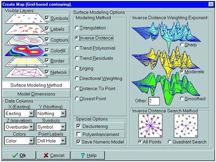
Gridding Tools: Reads X, Y, and Z data from the data sheet. Gridding algorithms: inverse distance, with optional radial searching and directional weighting, triangulation, closest point, kriging, trend surface analysis, trend surface residuals, distance to point. Grid utilities: statistics computations, arithmetic operations, filtering and logical operations, grid editor, grid export (see Export, below), grid import (from Surfer ASCII and binary, RockWorks DOS v.7, and ASCII formats), and slope/aspect analysis.

Mapping Tools: Map types: Point maps, non-gridded contour maps, and grid-based line contour, color-filled contour, labeled cell, strike and dip, uphill and downhill gradient, 3D surface mesh and raised contours. Point maps with customized symbols, and optional proportional scaling. Import commercial land grid data or create idealized land grid maps. Read survey data (distance/bearing/inclination): translate to XY and create map. Annotation with border tick marks and coordinate and axis labels. Legends with titles, scale bars, north arrow, logo, and/or comments. GIS information retrieval and editing of source data for map locations on the screen.

Solid Modeling: Reads XYZG data from RockWorks data sheet and linked downhole data files, or from existing XYZG data files (such as output from ProSect). Modeling methods: Inverse-distance (all points or octant-searched points), or closest point. Display solid models as solid block diagrams with optional removal of closest corner for interior viewing or selective unit display. Solid model options: statistical computations, arithmetic operations, model editing, extraction and insertion of 2-D horizontal or vertical "slices" as grid files. Other tools: model smoothing and filtering based on data range, polygon overlays, distance from control points. Boolean models created and filtered based on thickness of ore zones and stripping ratios; density conversions convert volumes to mass. Import solid model files in ProSect and ASCII formats. Export solid model files (see Export, below).

Volumetrics: Compute volumes of X, Y and Thickness values using simple triangulation technique. Or use grid-based volumetrics with thickness, stripping ratio, distance-to-point, polygon clipping, and up to 5 other data column filters; the grid-based volume or mass results can be output in a report and visualized in a 2 or 3D map. Advanced 3D volumetrics create solid models of "ore" versus "not-ore" and offer the 2D filters in 3-dimensions, with report and block diagram output of volumes or mass.

Stratigraphic Diagrams: Illustrate formation data as individual strip logs, hole-to-hole cross sections, and fence diagrams. Logs can include user-declared formation patterns, formation names, other text "zone" labels, scale bar, well name, and up to two curves and/or histograms of linked downhole data. Sections and fences can contain individual logs (with any / all of the individual log features), color- and/or pattern-filled panels, and reference annotation. Hang strata from any formation. User-controlled vertical exaggeration. Stratigraphic block models illustrate the 3D layering of formations, by creating 2D grid models of each formation and combining them into a 3D model. They can be illustrated as block diagrams with color-coded strata, and optional removal of the closest corner.

Statistics: 1 variable: Basic statistical computations, relative frequency histograms (with optional color-coding & annotation based on standard deviations), normalize or standardize a column of values. 2 variables: XY (scattergram) plots with optional point-to-point, smoothing, and linear regression annotations. 3 variables: Ternary plots with optional point density contours as lines and solid colors. Random number generators.

2D Feature Analysis: Rose diagrams (full or half) created from azimuth bearing or line endpoint data from the RockWorks data sheet. Data interpreted as uni-or bi-directional; may be rotated and filtered (by length and/or direction). Variable petal width, optional statistical legend and mean ray and error, and easy modification of title, reference rays and circles. Lineation gridding tools offer 2D and 3D maps of lineation frequencies, lengths, intersections, or a combination, reported as real number, normalized, or standardized values. Lineation maps, arrow maps, and strike&dip maps illustrate lineations and planes on a 2D maps. Compute azimuth, line length, and lineation midpoint for line endpoint data. Movement analysis computes direction, distance, inclination, and velocity data from X, Y, Z, and time data. Import DXF Line and Polyline entities into the data sheet.

3D Feature Analysis: Stereonet diagrams created from strike and dip (or dip-direction, dip-angle) data; plot linear, planar, or rake features. Planar data plotted as great circles or pole (normal). Unique symbols for each sample or groups of samples. Mean directional vectors, statistics, symbol index, and legend. Optional contours and/or color-filled contours to illustrate point density; density grid computed using step function or spherical Gaussian technique. Other options: rotation of planar data, computation of planar intersection lineations, conversion of rake information to lineations. Equal area (Schmidt) or equal angle (Wulff) projections.

Hydrology: Compute drawdown for a single well using the Theis equation and display as report and/or diagram. Compute drawdown for multiple pumping or injection wells listed in data sheet (also using Theis equation), display as 2D or 3D potentiometric surface map.

Digitizing: Digitizing of points and individual lines directly into the data sheet, using an electronic digitizing tablet (not supplied with program). Requires installation of the "Wintab32" driver supplied by the digitizer manufacturer.

Coordinate Conversions: Translate XY coordinates listed in RockWorks data sheet: Longitude / latitude to/from UTM (feet or meters), decimal degrees to/from degree-minute-second, polar (bearing and distance) to/from XY. Also convert azimuth bearings to quadrant, quadrant to azimuth bearing. Rescale, rotate, and shift XY coordinates.

Geological Tools: Three-point contouring, periodic table of the elements, geologic time scale, structural and trigonometric computations, geometry computations, measurement unit conversions (length, area, mass, etc.), financial utilities.

Rock Works main text
2or3D Feature Analysis