 | Raster & Vector GIS Analysis |
Figure 1.1-1. Spatial Analysis and Spatial Statistics are extensions of traditional ways of analyzing mapped data |
Figure 2.1-1. Calculating the total number of houses within a specified distance of each map location generates a housing density surface |
Figure 2.1-2. Spatial Data Mining techniques can be used to derive predictive models of the relationships among mapped data |
Figure 2.2-1. Map Analysis techniques can be used to identify suitable places for a management activity |
Figure 3.0-1. Grid-based data can be displayed in 2D/3D lattice or grid forms |
Figure 3.1-1. A map stack of individual grid layers can be stored as separate files or in a multi-grid table |
Figure 3.2-1. Map values are characterized from two broad perspectivesŚnumeric and geographicŚthen further refined by specific data types. |
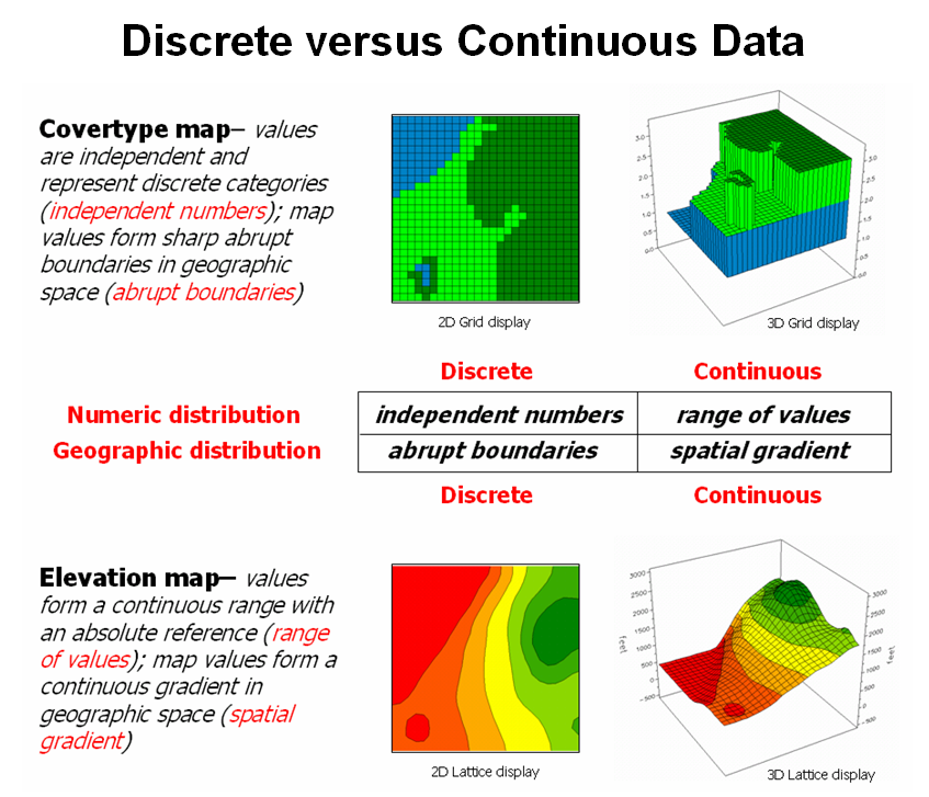
Figure 3.2-2. Discrete and Continuous map types combine the numeric and geographic characteristics of mapped data. |
Figure 3.3-1. 3D display ōpushes-upö the grid or lattice reference frame to the relative height of the stored map values. |
Figure 3.4-1. Comparison of different 2D contour displays using Equal ranges, Equal Count and +/-1 Standard deviation contouring techniques |
Figure 4.1.1-1. Spatial interpolation involves fitting a continuous surface to sample points. |
Figure 4.1.2-1. Variogram plot depicts the relationship between distance and measurement similarity (spatial autocorrelation). |
Figure 4.1.3-1. Spatial comparison of a whole-field average and an IDW interpolated map |
Figure 4.1.3-2. Spatial comparison of IDW and Krig interpolated maps |
Figure 4.1.4-1. A residual analysis table identifies the relative performance of average, IDW and Krig estimates |
Figure 4.2.1-1. Map surfaces identifying the spatial distribution of P,K and N throughout a field |
Figure 4.2.1-2. Geographic space and data space can be conceptually linked |
Figure 4.2.1-3. A similarity map identifies how related the data patterns are for all other locations to the pattern of a given comparison location |
Figure 4.2.2-1. Level-slice classification can be used to map sub-groups of similar data patterns. |
Figure 4.2.3-1. Map clustering identifies inherent groupings of data patterns in geographic space |


Analysis
n Identify shrub
locations
Ģ 1x1 m resolution
from 1991 image
is sufficient to
resolve individual
colonizing
shrubs
Elevations
n The NOAA Airborne
LIDAR Assessment
of Coastal Erosion
(ALACE) program
flew over Hog
Island in 1997
Ģ 15 cm vertical
resolution
Ģ 5 m horizontal
resolution
Compare actual shrub locations with a
similar number randomly chosen
locations
Ģ 150 shrub locations were identified
¢Only one shrub per clump identified to avoid
effects of vegetative growth
Ģ 150 random locations in the vicinity of the
shrubs were identified
The elevations of shrub
and random locations
are used to statistically
assess the use of dune
and swale regions by
colonizing shrubs
Images ¢ a special type of
raster
Digital Representation of Images
n To understand how image processing
works, it is first necessary to understand
how digital images are represented in
the computer
n Images are stored in RASTER form
Each pixel takes on a ōradiometric
intensityö or ōbrightness valueö
Ģ Pixel values typically vary between 0 and
255 (the maximum value one byte of data
can take)
Color Images
n Color images are differentiated from black
and white images because they have more
than one ōbandö
Ģ Bands in a color image typically represent the
ōbrightnessö in different parts of the spectrum
¢ For example, one band may depict the brightness in the
blue part of the spectrum while another band represents
brightness in the infrared band
Ģ When bands are combined, we can display color
images
Multispectral Imagery
n Images with more than one band are
referred to as ōmultispectralö
Ģ Although you can only display 3 bands at a
time (only have red, green and blue ōgunsö
in your monitor), images may have many
more bands
Ģ Most multispectral satellite images have 3-
10 bands
Ģ Some images can have up to 200 or more
bands and are referred to as
ōhyperspectralö
Image Displays donÆt all need to
be of a single image
n One way of doing a change analysis is
to use the same band from images
taken at different TIMES
n Thus instead of multi-spectral, we have
multi-temporal displays
Pixel Values
n In our input images the individual pixel
has values that
Ģ Are continuous (usually over integer values
between 0 and 255)
Ģ Can be expressed as a vector or comma
separated numbers
¢ E.g. if for an individual pixel band 1= 20, band
2=30 and band 3=190, we could express that
as the vector (20,30,190)
Characteristics of Images
n Extent ¢ what is the land area that is represented in
the image? E.g., 120x60 km
n Spatial Resolution ¢ what are the dimensions of a
pixel? E.g., 2 m on a side
Ģ Note a high resolution image has a small pixel size
Ģ Sometimes spatial resolution is particular to specific bands in
an image
n Radiometric Resolution ¢ what range of brightness
values can be represented?
Ģ By far the most common is 8-bit (256 unique values)
Ģ Some images contain 12-bit (4096) or even 16-bit (65,536)
distinguishable levels
Creating Raster Data
Raster Data
Raster data can be created in a variety of
ways:
n Classification of an image to convert
brightness values into meaningful
classes
Ģ Unsupervised Classification
Ģ Supervised Classification
n Conversion of vector data to raster
Ģ Nearest Neighbor
Ģ Contouring
Remote Sensing to GIS
Maximum Likelihood Classification
n The Maximum Likelihood Classification
tool reads the signature file created by
ISO Cluster and produces
Ģ The raster output map
Ģ A raster that indicates how likely the
classification for each pixel was
Other Approaches
n In Supervised Classification you select
signatures manually, rather than having
ISO Cluster extract them for you
manually, otherwise the process is the
same
Converting from Raster to Vector
The conversion from raster to vector
varies in difficulty with the type of data
n POINTS and POLYGONS are relatively
easy (esp. for classified remote sensing
data)
n LINES are relatively hard
n ARCScan is a extension that helps to
create vector maps from scanned paper
maps
Ģ It can be a complicated and difficult
process!
Choosing between Raster and
Vector
n How dense is your collection of
measurements?
n Are they regularly distributed in a grid?
n Continuous vs categorical?
n Do you need to calculate any statistics
based on surrounding areas?
n Do you need to represent lines?
MODELLING AND ANALYSIS
Table of Contents (with Hyperlinks)
Topic
Page
1.0 Introduction
1.1 Mapping to Analysis of Mapped Data
1.2 Vector-based Mapping versus Grid-based Analysis
3
4
5
2.0 Fundamental Map Analysis Approaches
2.1 Spatial Statistics
2.2 Spatial Analysis
5
6
8
3.0 Data Structure Implications
3.1 Grid Data Organization
3.2 Grid Data Types
3.3 Grid Data Display
3.4 Visualizing Grid Values
9
11
12
14
16
4.0 Spatial Statistics Techniques
4.1 Surface Modeling
4.1.1 Point Samples to Map Surfaces
4.1.2 Spatial Autocorrelation
4.1.3 Benchmarking Interpolation Approaches
4.1.4 Assessing Interpolation Results
4.2 Spatial Data Mining
4.2.1 Calculating Map Similarity
4.2.2 Identifying Data Zones
4.2.3 Mapping Data Clusters
4.2.4 Deriving Prediction Maps
4.2.5 Stratifying Maps for Better Predictions
17
17
17
19
20
22
24
24
28
29
32
35
5.0 Spatial Analysis Techniques
5.1 Spatial Analysis Framework
5.2 Reclassifying Maps
5.3 Overlaying Maps
5.4 Establishing Distance and Connectivity
5.5 Summarizing Neighbors
39
41
42
46
48
55
6.0 GIS Modeling Frameworks
6.1 Suitability Modeling
6.1.1 Binary Model
6.1.2 Ranking Model
6.1.3 Rating Model
6.2 Decision Support Modeling
6.2.1 Routing Procedure
6.2.2 Identifying Corridors
6.2.3 Calibrating Routing Criteria
6.2.4 Weighting Criteria Maps
6.2.5 Transmission Line Routing Experience
6.3 Statistical Modeling
6.3.1 Elements of Precision Agriculture
GIS Modeling and Analysis
.0 Introduction
1.1 Mapping to Analysis of Mapped Data
1.2 Vector-based Mapping versus Grid-based Analysis
3
4
5
2.0 Fundamental Map Analysis Approaches
2.1 Spatial Statistics
2.2 Spatial Analysis
5
6
8
3.0 Data Structure Implications
3.1 Grid Data Organization
3.2 Grid Data Types
3.3 Grid Data Display
3.4 Visualizing Grid Values
9
11
12
14
16
4.0 Spatial Statistics Techniques
4.1 Surface Modeling
4.1.1 Point Samples to Map Surfaces
4.1.2 Spatial Autocorrelation
4.1.3 Benchmarking Interpolation Approaches
4.1.4 Assessing Interpolation Results
4.2 Spatial Data Mining
4.2.1 Calculating Map Similarity
4.2.2 Identifying Data Zones
4.2.3 Mapping Data Clusters
4.2.4 Deriving Prediction Maps
4.2.5 Stratifying Maps for Better Predictions
17
17
17
19
20
22
24
24
28
29
32
35
5.0 Spatial Analysis Techniques
5.1 Spatial Analysis Framework
5.2 Reclassifying Maps
5.3 Overlaying Maps
5.4 Establishing Distance and Connectivity
5.5 Summarizing Neighbors
39
41
42
46
48
55
6.0 GIS Modeling Frameworks
6.1 Suitability Modeling
6.1.1 Binary Model
6.1.2 Ranking Model
6.1.3 Rating Model
6.2 Decision Support Modeling
6.2.1 Routing Procedure
6.2.2 Identifying Corridors
6.2.3 Calibrating Routing Criteria
6.2.4 Weighting Criteria Maps
6.2.5 Transmission Line Routing Experience
6.3 Statistical Modeling
6.3.1 Elements of Precision Agriculture
6.3.2 The Big Picture
Raster & Vector GIS
GIS Modeling and Analysis
GIS Modeling and Analysis text